Summary
The Compare Tool is a versatile and powerful analysis capability in Voyager that can be used to assess overall dimensional deviations in a variety of applications. For example:- Comparing a scan of a part with the CAD model that was used to make it to understand both global and local dimensional deviations.
- Comparing two scans of the same part to characterize wear over time or the impact of accelerated lifetime testing.
- Comparing different instances of the same part to quantify differences between injection mold cavities or differences between different vendors.
Preparing Your CAD (or Nominal) Mesh
The Nominal Mesh represents either design intent, in the case of comparing a scan to CAD, or the state that you want to compare the analysis Mesh to (before use in the case of wear testing, for example). If creating a Nominal Mesh from a CAD tool:1
Isolate Your Part
In your CAD tool, isolate the body that you would like to use for the analysis.
2
Export the body as an STL
Ensure that the mesh contains enough polygons to properly resolve curves. CAD tools often default to a low polygon count when exporting CAD models (left) - the middle image illustrates a low polygon count while the right image illustrates a sufficiently high polygon count. If you have access to the mesh generation parameters in your CAD tool, set the “surface deviation” to a value of 0.001 mm or lower. This will reduce error from tessellating the CAD model.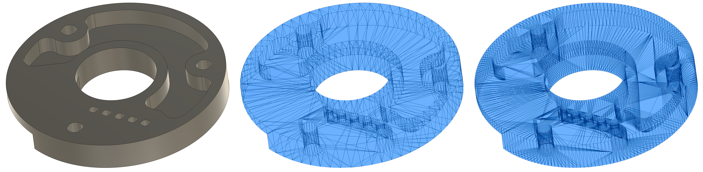
3
Import the STL into your Voyager Project.
Use the Import Tool to load your external Mesh into the Project. Be sure to set the units to the same units that were used in the CAD tool that you exported from.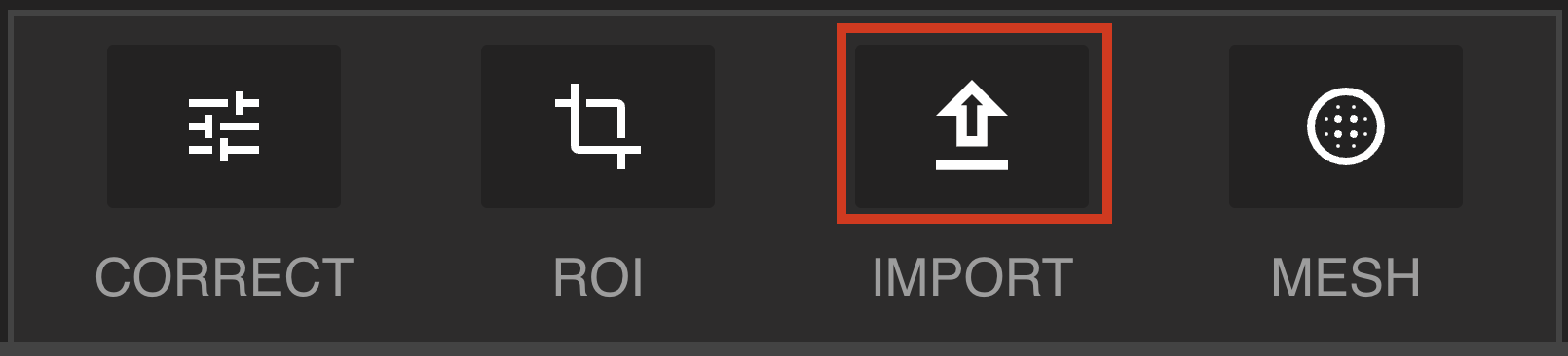
Preparing Your Analysis Mesh
The Analysis Mesh or Mesh to Analyze is the Mesh that you would like to characterize. Typically this Mesh is generated in Voyager from CT scan data using Voyager’s Mesh Tool. Meshes from third-party scanners (like structured light scanners) can also be imported and used as an Analysis Mesh.Running the Workflow
1
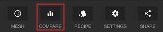
Select the Compare button in the Toolbar
2
Select the Mesh you would like to analyze

3
Select your nominal Mesh

4
Coarsely align the Meshes
Using the rotation handles in the view ports, rotate the analysis Mesh until it is approximately aligned with the nominal Mesh. This does not have to be perfect as we will next run a fine automatic alignment to more precisely align the two Meshes.
5
Run auto-alignment
Auto alignment performs a global best fit alignment. This works well when the deviations between parts are small, but may require some manual adjustments if there are large differences between parts or if it is important to align to a specific feature or datum.
6
Submit the comparison
Once you are satisfied with your alignment, click “Submit” to send the analysis to the Lumafield Cloud for computation. Results are typically available within 1-10 minutes.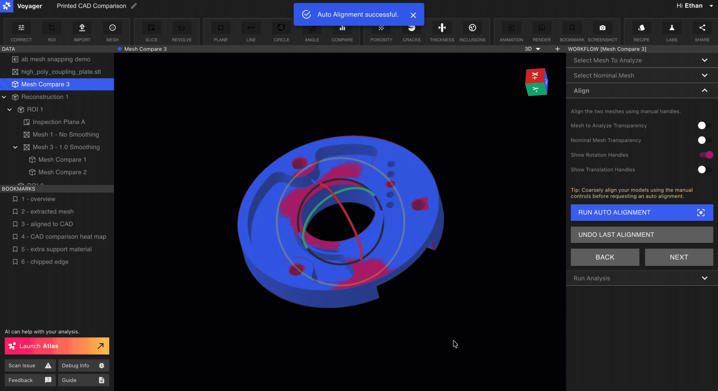
Visualizing and Interpreting Results
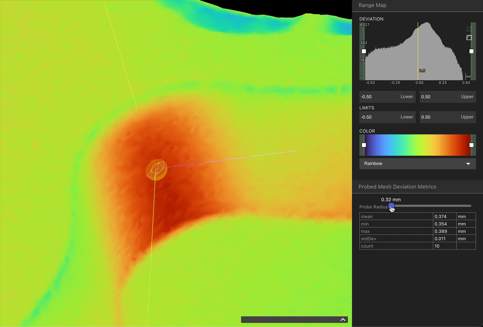
3D
The Compare Tool maps deviations between the Analysis and the Nominal meshes onto the Analysis Mesh and displays a heatmap visualization. Red corresponds to positive deviations, meaning regions in which the analysis Mesh deviates away from the nominal Mesh. Blue corresponds to areas with negative deviation, ie, material is absent relative to the nominal Mesh.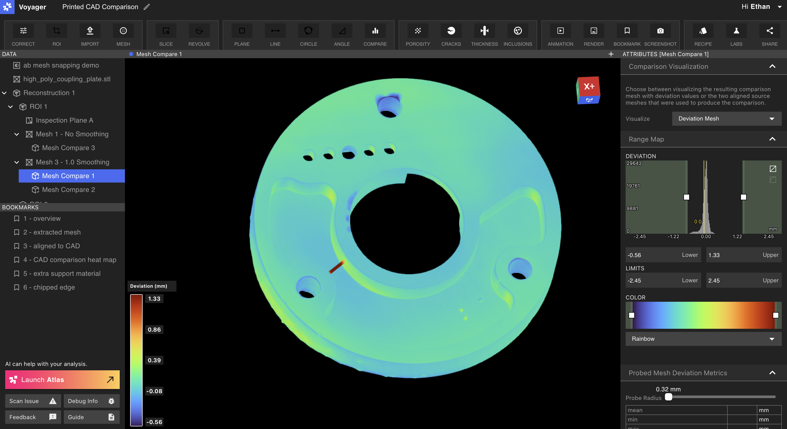
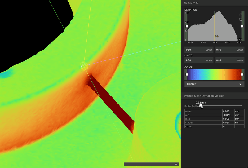
Probe Tool
Clicking anywhere on a Compare analysis result will activate the probe Tool, measuring the deviation at that location. The mean deviation and the number of polygons being sampled by the probe are displayed in the lower left hand corner, near the color bar.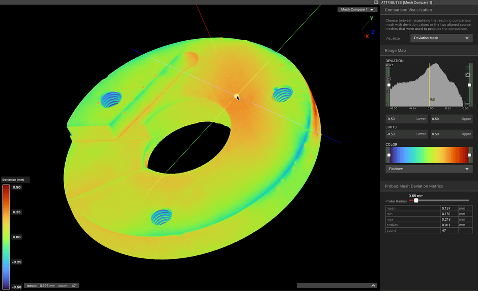
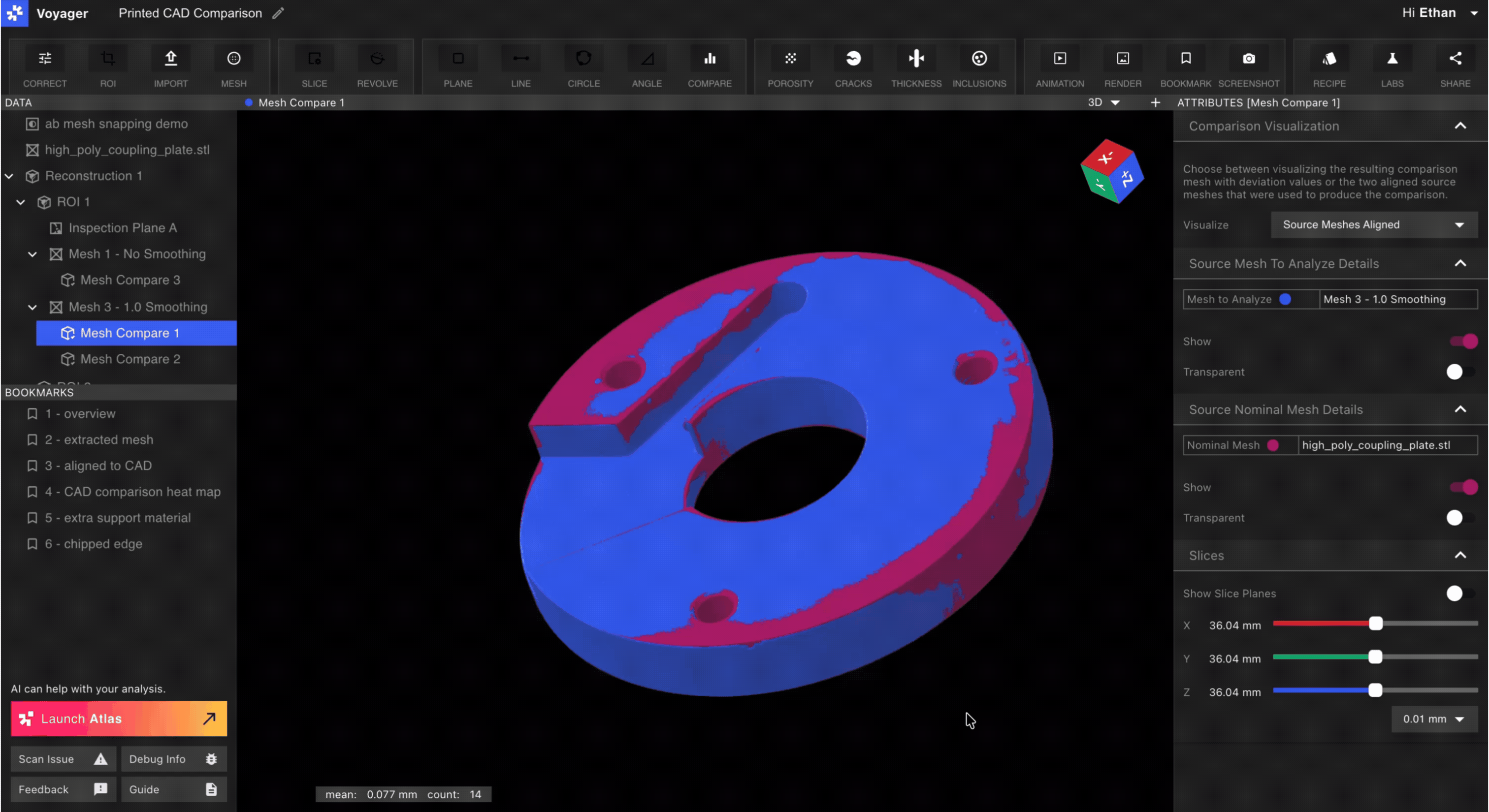
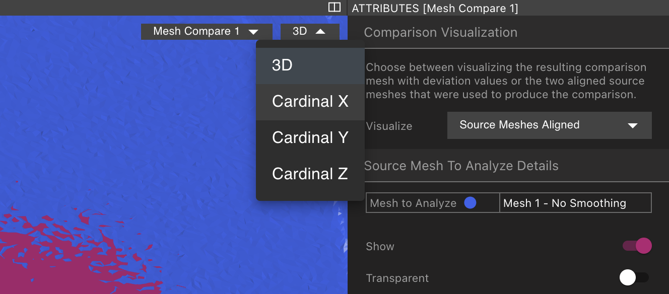
2D
Comparative analysis results can also be reviewed in 2D. To enter 2D mode, select “Source Meshes Aligned” from the “Visualize” dropdown menu in the Attributes Panel.
Troubleshooting and Common Problems
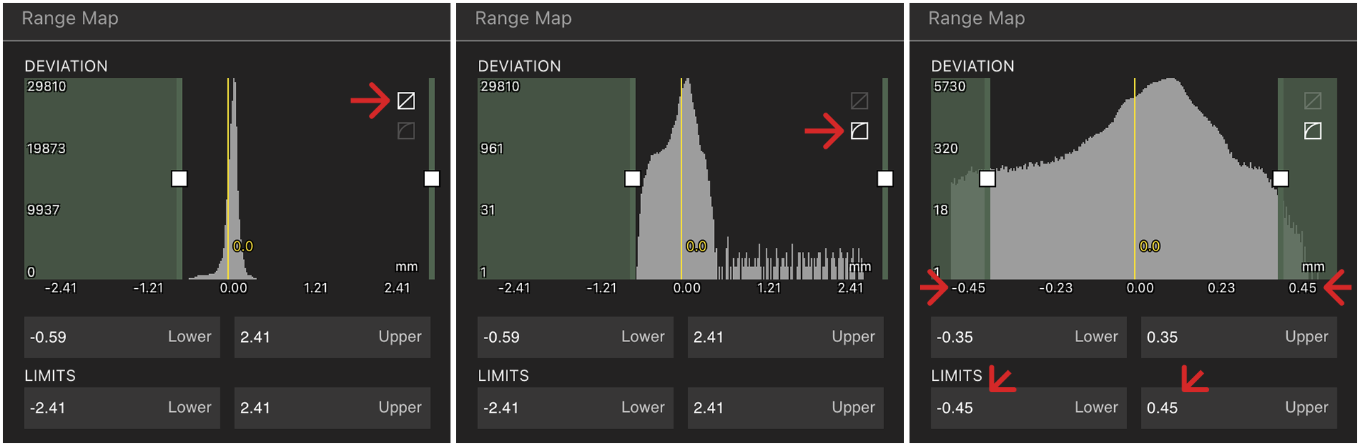
Histogram just has one skinny spike
Every vertex in a Mesh is included in a comparison analysis, so if your analysis Mesh has extraneous pieces of Mesh or has voids (say in the case of a casting or injection molded component) or stray pieces of Mesh, distances will be computed between the nominal surface and these surfaces as well. The impact of this effect can be reduced via two methods:- Use the rangemapper to exclude outliers. This can be accomplished by switching the rangemapper to log mode (upper right hand button) and then specifying new limits that better fit the distribution of deviations.
- Export the analysis Mesh and clean it in a 3rd party Tool like Meshlab to remove disconnected bodies or to trim extraneous surfaces. Re-Upload and re-compute your analysis.
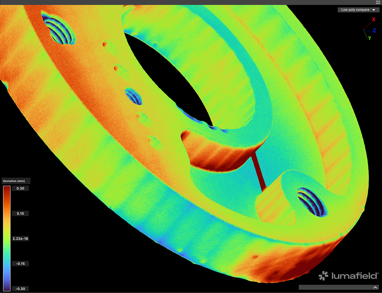
”Stripes” in the comparison results
“Stripes” in a comparative analysis result like the example below are due to too low a polygon count on the nominal mesh. If using a CAD tool to export an STL of the nominal part, increase the number of polygons. If using a scan mesh, re-export with a higher polygon count.